viewORCA Manual

There are several modules available for viewing ORCA calculations. This webpage describes all the modules available in viewORCA:

Info

You can view all the module available in viewORCA by typing viewORCA --help into the terminal:

username@computer name Desktop % viewORCA --help
usage: viewORCA [-h] [-T] {help,opt,scan,neb,neb_snap,irc,multi,move_com,append} ...

Program for viewing jobs from ORCA

optional arguments:
  -h, --help            show this help message and exit
  -T, --traceback

Sub-commands:
  {help,opt,scan,neb,neb_snap,irc,multi,move_com,append}
    help                Help for sub-command.
    opt                 This module allows the user to view the output of an ORCA geometric optimisation job visually.
    scan                This module allows the user to view the output of an ORCA SCAN job visually.
    neb                 This module allows the user to view the output of an ORCA Nudged Elastic Band (NEB) job visually.
    neb_snap            This module allows the user to view the progress of an ORCA Nudged Elastic Band (NEB) job (as it is running or after it has run) by viewing the energy profiles of all the iterations of the NEB optimisation job.
    irc                 This module allows the user to view the output of an ORCA Intrinsic Reaction Coordinate (IRC) job visually.
    multi               This module allows the user to obtain the number of electrons in the system of interest, and therefore obtain the possible multiplicities that the system could be in.
    move_com            This module allows the user to move the centre of mass of a system.
    append              This module allows the user to append a set of chemical systems together.

viewORCA opt: View Geometric Optimisation Calculation

This module is designed to allow the user to view the output of an ORCA geometric optimisation job visually.

To use this module:

1. In the terminal, change directory into the directory containing your geometric optimisation job, and
2. type viewORCA opt into the terminal.

# First, change directory into the folder containing your ORCA geometric optimisation job.
cd path_to_geometric_optimisation_job

# Second, run "viewORCA opt".
viewORCA opt

viewORCA opt will extract information from the ORCA_INPUT_FILENAME_trj.xyz file and show the images of the optimisation, along with the energy profile of the optimisation.

• For this reason, you MUST have the ORCA_INPUT_FILENAME_trj.xyz file in your geometric optimisation folder for viewORCA opt to work.
• The prefix ORCA_INPUT_FILENAME is the same prefix you gave to your ORCA input file (being ORCA_INPUT_FILENAME.inp).

This program will also create an xyz file called ORCA_INPUT_FILENAME_OPT_images.xyz that contains the images and the energy profile from the optimisation.

• You can view this by typing ase gui ORCA_INPUT_FILENAME_OPT_images.xyz into the terminal.

  ase gui ORCA_INPUT_FILENAME_OPT_images.xyz
  

Optional inputs for viewORCA opt include:

• --path: This is the path to the folder containing the ORCA optimisation calculation. If not given, the default path is the current directory you are in.
• --view: If tag indicates if you want to view the ASE GUI for the optimisation job immediate after this program has run. By default this is True. If you only want to create the ORCA_INPUT_FILENAME_OPT_images.xyz file and not view it immediately, set this to False.
  • Setting this to False is ideal if you are running viewORCA on an HPC, where ase gui windows may be more responsive if ase gui is run from your own computer rather than directly on the HPC.
  • You can view ORCA_INPUT_FILENAME_OPT_images.xyz on your computer by typing the following into the terminal: ase gui ORCA_INPUT_FILENAME_OPT_images.xyz.

Example

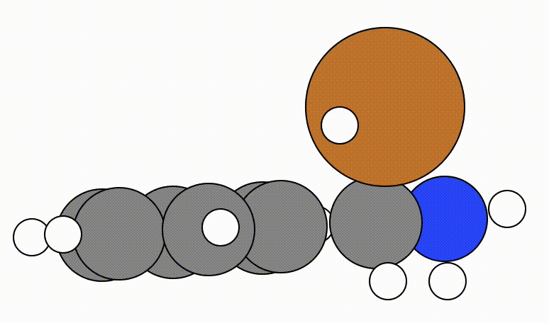
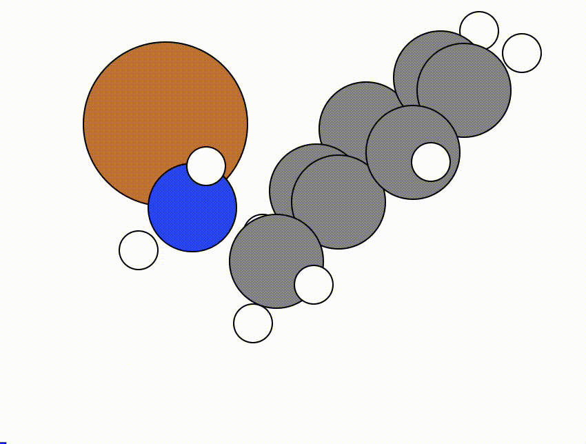
An example of a geometric optimisation viewed using viewORCA opt is shown below, along with the energy profile for this optimisation. This example is given in Examples/viewORCA_opt

NEB Images from a geometric optimisation

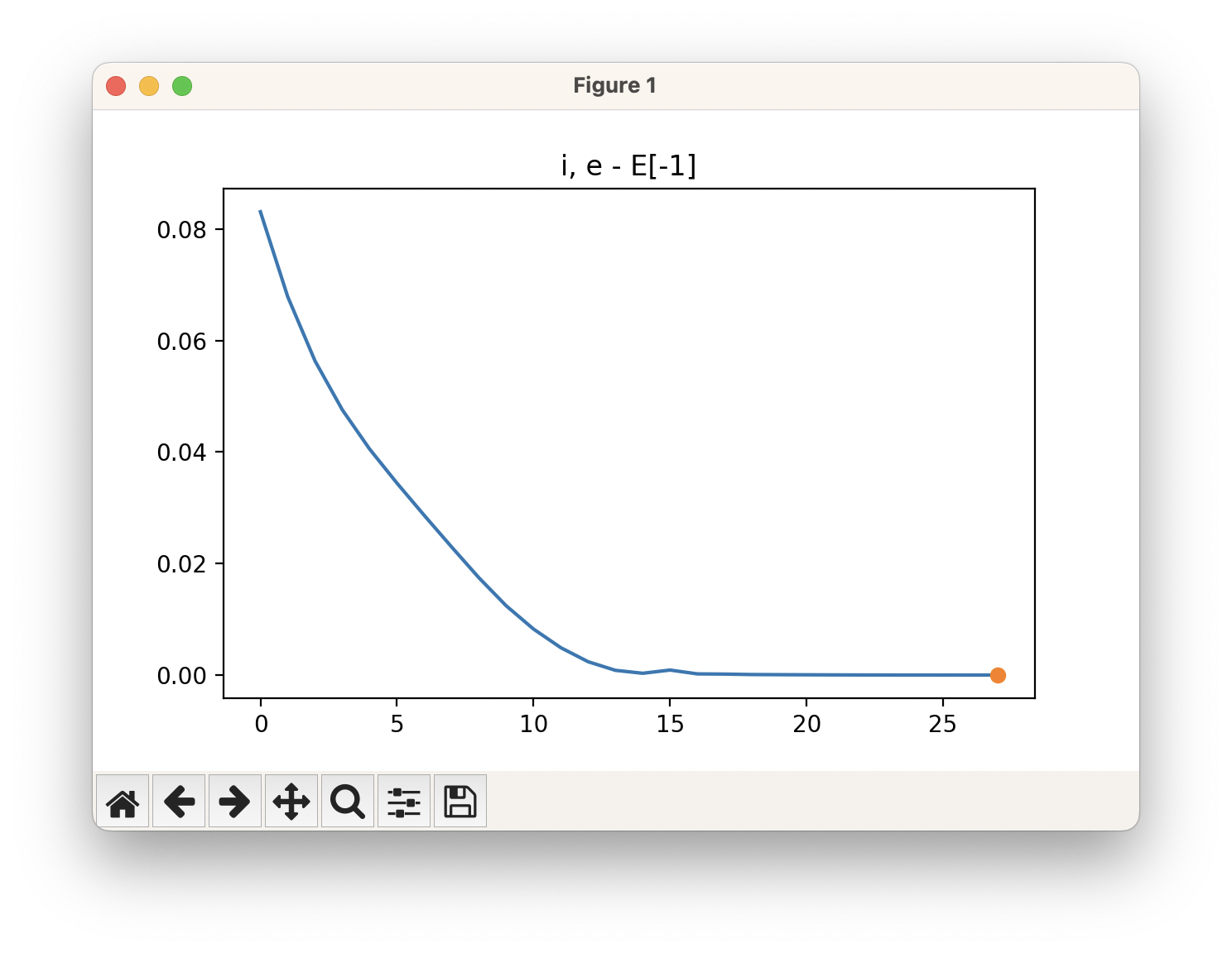
The energy profile for this example is given below:

Energy Profile from a geometric optimisation

viewORCA scan: View SCAN Calculation

This module is designed to allow the user to view the output of an ORCA SCAN job visually.

To use this module:

1. In the terminal, change directory into the directory containing your SCAN job, and
2. type viewORCA scan into the terminal.

# First, change directory into the folder containing your ORCA SCAN job.
cd path_to_SCAN_job

# Second, run "viewORCA scan".
viewORCA scan

Note

If you needed to restart your SCAN calculation part-way though the calculation for some reason and have multiple SCAN calculations that consectively run one after the other, you can run these sets of calculations together through viewORCA scan

• viewORCA scan will cellotape these calculations together so you can see the SCAN images together, and the full energy profile in one plot.

To use viewORCA scan in this way, make sure that your SCAN jobs are placed in separate folders called SCAN_1, SCAN_2, SCAN_3, so on and so on. viewORCA scan will paste these together in numerical order of these folders.

• Click here to learn more about this from the Procedure for Investigating Chemical Mechanisms with ORCA tutorial.

viewORCA scan will show the images of the SCAN calculation, along with the energy profile of the SCAN calculation.

• This program will also create an xyz file called SCAN_images.xyz that contains the images and the energy profile from the SCAN calculation. You can view this by typing ase gui SCAN_images.xyz into the terminal.

  ase gui SCAN_images.xyz
  

Optional inputs for viewORCA scan include:

• --path: This is the path to the folder containing the ORCA SCAN calculation. If not given, the default path is the current directory you are in.
• --view: If tag indicates if you want to view the ASE GUI for the SCAN job immediate after this program has run. By default this is True. If you only want to create the SCAN_images.xyz file and not view it immediately, set this to False.
  • Setting this to False is ideal if you are running viewORCA on an HPC, where ase gui windows may be more responsive if ase gui is run from your own computer rather than directly on the HPC.
  • You can view SCAN_images.xyz on your computer by typing the following into the terminal: ase gui SCAN_images.xyz.

Example

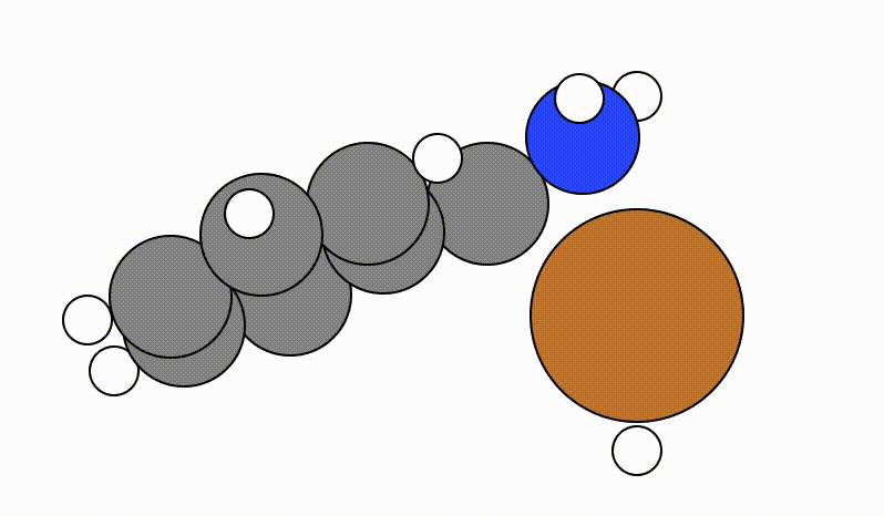
An example of a SCAN calculation viewed using viewORCA scan is shown below, along with the energy profile for this SCAN calculation. This example is given in Examples/viewORCA_scan

NEB Images from a SCAN calculation

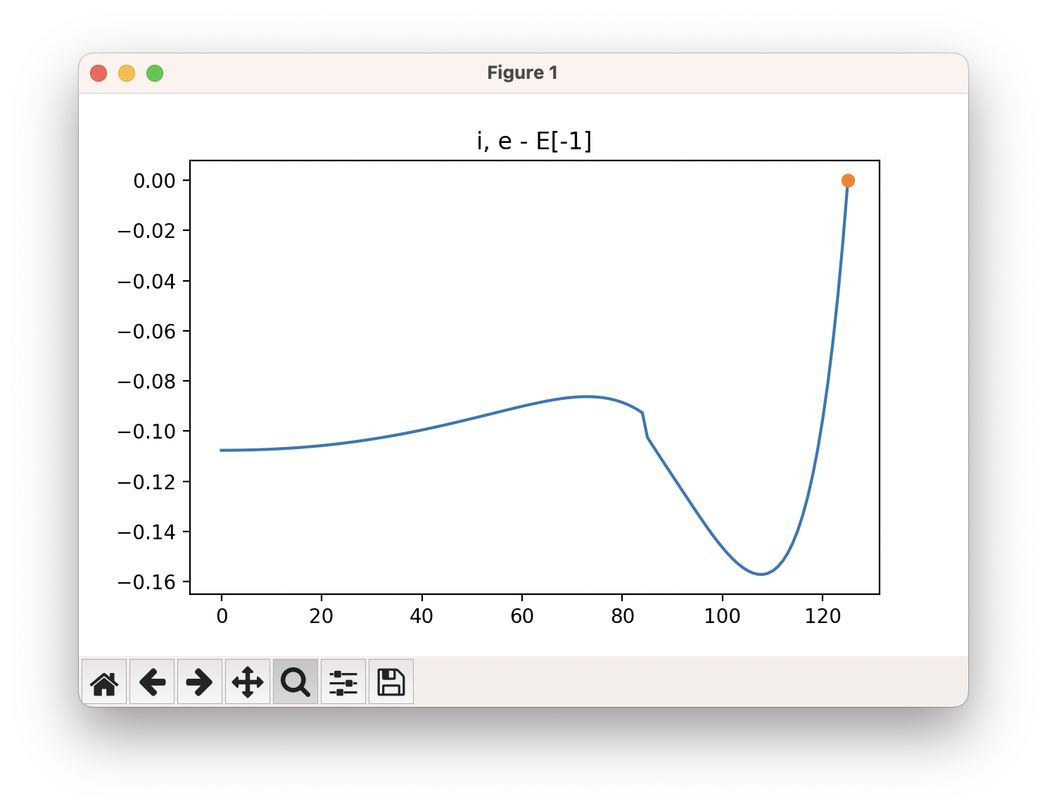
The energy profile for this example is given below:

Energy Profile from a SCAN calculation

viewORCA neb: View Nudged Elastic Band (NEB) Calculation

This module is designed to allow the user to view the output of an ORCA NEB job visually.

To use this module:

1. In the terminal, change directory into the directory containing your NEB job, and
2. type viewORCA neb into the terminal.

# First, change directory into the folder containing your ORCA NEB job.
cd path_to_NEB_job

# Second, run "viewORCA neb".
viewORCA neb

viewORCA neb will extract information from the ORCA_INPUT_FILENAME_MEP_trj.xyz file and show the images of the NEB calculation, along with the energy profile of the NEB calculation.

• For this reason, you MUST have the ORCA_INPUT_FILENAME_MEP_trj.xyz file in your NEB calculation folder for viewORCA neb to work.
• The prefix ORCA_INPUT_FILENAME is the same prefix you gave to your ORCA input file (being ORCA_INPUT_FILENAME.inp).

This program will also create an xyz file called ORCA_INPUT_FILENAME_NEB_images.xyz that contains the images and the energy profile from the NEB calculation.

• You can view this by typing ase gui ORCA_INPUT_FILENAME_NEB_images.xyz into the terminal.

  ase gui ORCA_INPUT_FILENAME_NEB_images.xyz
  

Optional inputs for viewORCA neb include:

• --path: This is the path to the folder containing the ORCA NEB calculation. If not given, the default path is the current directory you are in.
• --view: If tag indicates if you want to view the ASE GUI for the NEB job immediate after this program has run. By default this is True. If you only want to create the ORCA_INPUT_FILENAME_NEB_images.xyz file and not view it immediately, set this to False.
  • Setting this to False is ideal if you are running viewORCA on an HPC, where ase gui windows may be more responsive if ase gui is run from your own computer rather than directly on the HPC.
  • You can view ORCA_INPUT_FILENAME_NEB_images.xyz on your computer by typing the following into the terminal: ase gui ORCA_INPUT_FILENAME_NEB_images.xyz.

Example

An example of a NEB calculation viewed using viewORCA neb is shown below, along with the energy profile for this NEB calculation. This example is given in Examples/viewORCA_neb_and_neb_snap

NEB Images from a NEB calculation

The energy profile for this example is given below:

Energy Profile from a NEB calculation

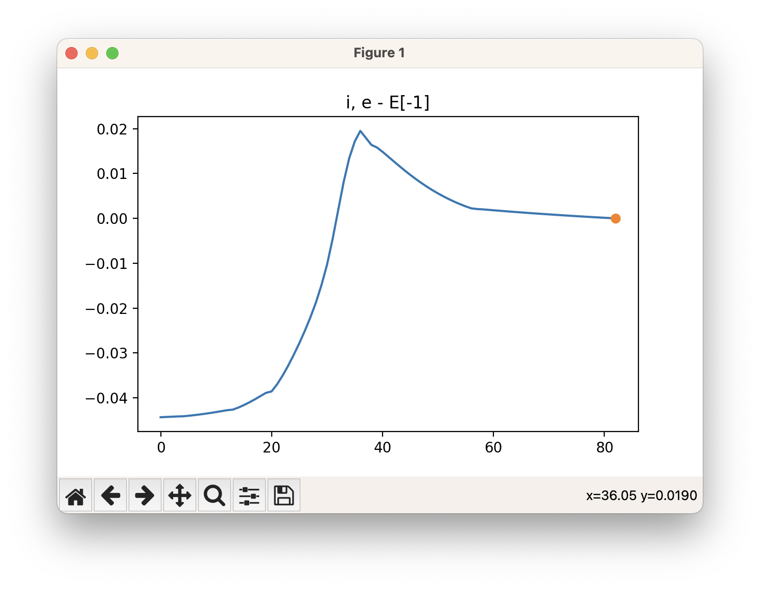
viewORCA neb_snap: View NEB Optimisation Process

This module is designed to allow the user to view the energy profile of all the iterations performed during the NEB optimisation process. This module is an adaptation of neb_snapshots.py by Vilhjálmur Ásgeirsson and Benedikt Orri Birgirsson of the Universiy of Iceland.

• It is helpful to view this as your NEB calculation is running to check if there are any issues occurring as ORCA us running the NEB calculation.

To use this module:

1. In the terminal, change directory into the directory containing your NEB job, and
2. type viewORCA neb_snap into the terminal.

# First, change directory into the folder containing your ORCA NEB job.
cd path_to_NEB_job

# Second, run "viewORCA neb_snap".
viewORCA neb_snap

viewORCA neb_snap will extract information from the ORCA_INPUT_FILENAME.interp file and create plots of the energy profiles of all the iterations of the NEB optimisation process.

• For this reason, you MUST have the ORCA_INPUT_FILENAME.interp file in your NEB calculation folder for viewORCA neb_snap to work.
• The prefix ORCA_INPUT_FILENAME is the same prefix you gave to your ORCA input file (being ORCA_INPUT_FILENAME.inp).

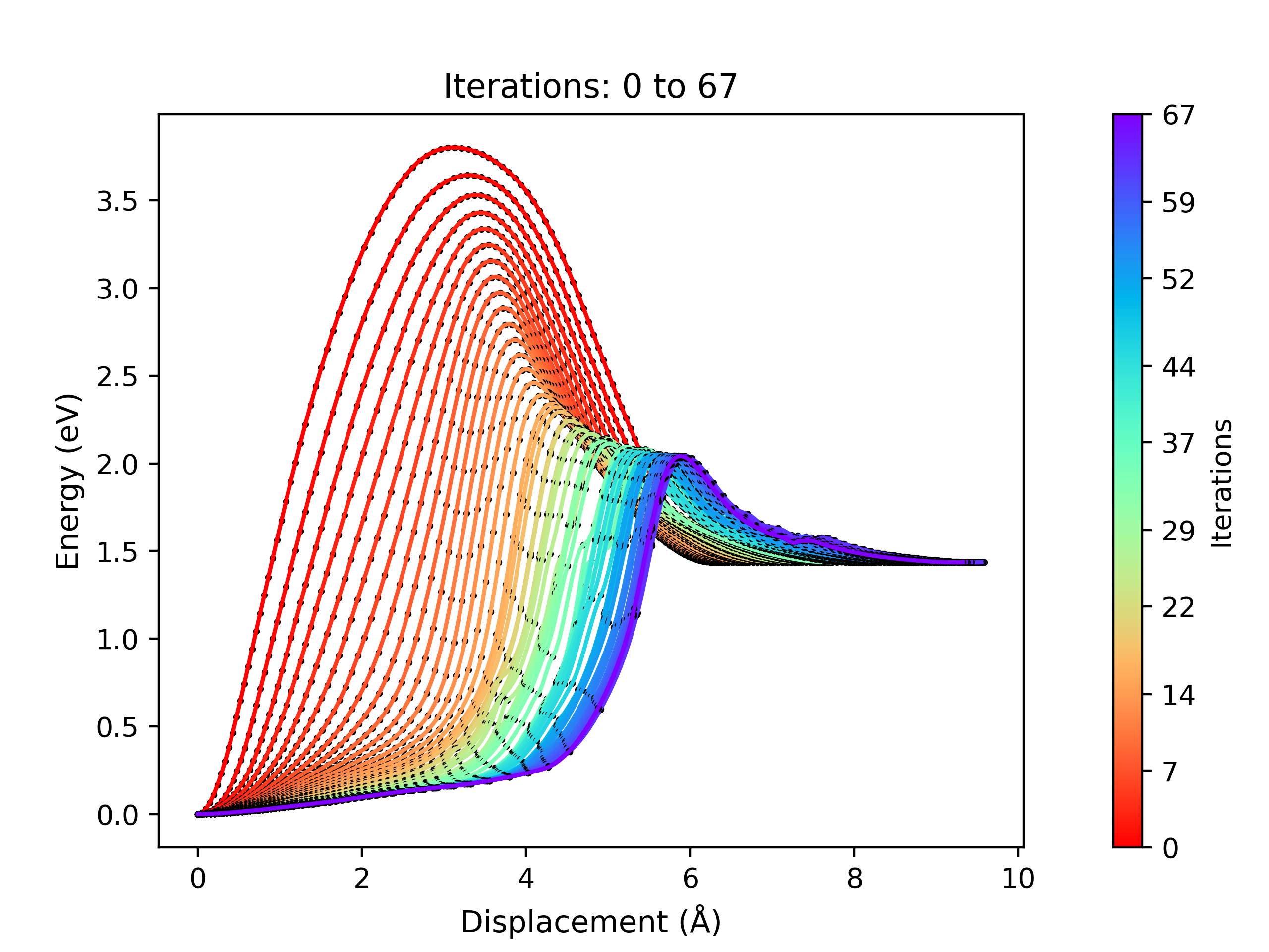
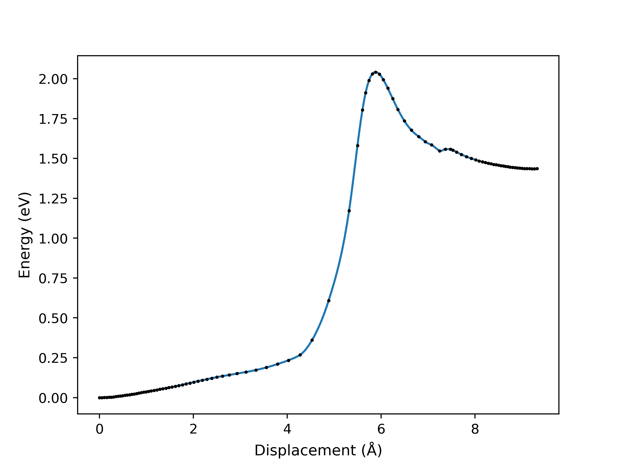
viewORCA neb_snap will create two png files containing the energy profiles of the NEB calculation:

• ORCA_INPUT_FILENAME_NEB_optimization.png: This plot displays the NEB energy profiles of all iterations performed during the NEB optimisation process.
• ORCA_INPUT_FILENAME_NEB_last_iteration.png: This plot shows the energy profile of the last iteration performed from the NEB optimisation process.

Optional inputs for viewORCA neb_snap include:

• --path: This is the path to the folder containing the ORCA NEB calculation. If not given, the default path is the current directory you are in.
  • You can also provide the path to the .interp file you want to process if you want to process a specific .interp file of interest. This file must end with the .interp suffix.

Example

An example of a NEB optimisation calculation viewed using viewORCA neb_snap is shown below, along with the energy profile of the last iteration for this NEB calculation. This example is given in Examples/viewORCA_neb_and_neb_snap

Energy Profile of each NEB optimisation iteration performed by ORCA. This is given by the 'ORCA_INPUT_FILENAME_NEB_optimization.png' file.

Energy Profile of each NEB optimisation iteration performed by ORCA. This is given by the 'ORCA_INPUT_FILENAME_NEB_last_iteration.png' file.

viewORCA irc: View Intrinsic Reaction Coordinate (IRC) Calculation

This module is designed to allow the user to view the output of an ORCA IRC job visually.

To use this module:

1. In the terminal, change directory into the directory containing your IRC job, and
2. type viewORCA irc into the terminal.

# First, change directory into the folder containing your ORCA IRC job.
cd path_to_geometric_optimisation_job

# Second, run "viewORCA irc".
viewORCA irc

viewORCA irc will extract information from the ORCA_INPUT_FILENAME_IRC_Full_trj.xyz file and show the images of the IRC calculation, along with the energy profile of the IRC calculation.

• For this reason, you MUST have the ORCA_INPUT_FILENAME_IRC_Full_trj.xyz file in your NEB calculation folder for viewORCA neb to work.
• The prefix ORCA_INPUT_FILENAME is the same prefix you gave to your ORCA input file (being ORCA_INPUT_FILENAME.inp).

This program will also create an xyz file called ORCA_INPUT_FILENAME_IRC_images.xyz that contains the images and the energy profile from the IRC calculation.

• You can view this by typing ase gui ORCA_INPUT_FILENAME_IRC_images.xyz into the terminal

  ase gui ORCA_INPUT_FILENAME_IRC_images.xyz
  

Optional inputs for viewORCA irc include:

• --path: This is the path to the folder containing the ORCA IRC calculation. If not given, the default path is the current directory you are in.
• --view: If tag indicates if you want to view the ASE GUI for the IRC job immediate after this program has run. By default this is True. If you only want to create the SCAN_images.xyz file and not view it immediately, set this to False.
  • Setting this to False is ideal if you are running viewORCA on an HPC, where ase gui windows may be more responsive if ase gui is run from your own computer rather than directly on the HPC.
  • You can view ORCA_INPUT_FILENAME_IRC_images.xyz on your computer by typing the following into the terminal: ase gui ORCA_INPUT_FILENAME_IRC_images.xyz.

Example

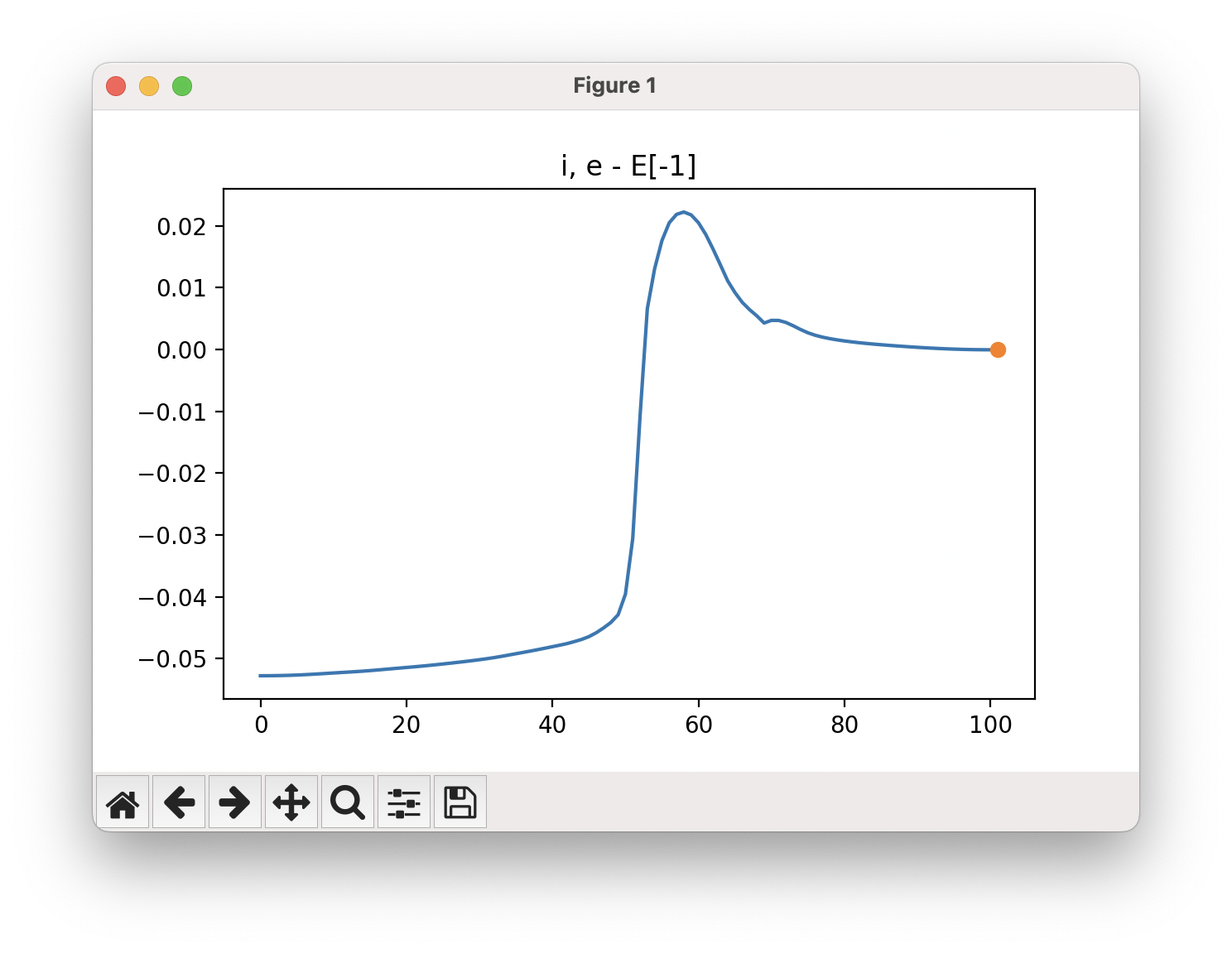
An example of a IRC calculation viewed using viewORCA irc is shown below, along with the energy profile for this IRC calculation. This example is given in Examples/viewORCA_irc

NEB Images from a IRC calculation

The energy profile for this example is given below:

Energy Profile from a IRC calculation

viewORCA multi: Obtain Possible Electron Multiplicities for your System

One of the inputs that you need to give to your ORCA input .inp file is the multiplicity of the system. The multiplicity indicates the total electron spin of your system. The value of the muliticity is based on the number of electrons are in your system, where the multiplicity is based on the \(M = 2S + 1\) rule:

• If you have an even number of electrons in your system, the multiplicity will be an odd number. The lowest value multiplicity is 1.
• If you have an odd number of electrons in your system, the multiplicity will be an even number. The lowest value multiplicity is 2 (It can not be 0).

If you want to easily figure out if you should have an even or odd multiplicity, the viewORCA multi will determine the number of electrons your system has, and from this indicate if your multiplicity will be even or odd.

To use this module:

1. In the terminal, change directory into the directory containing your geometric optimisation job, and

2. type viewORCA multi filepath --charge=charge into the terminal, where:

   • filepath is the path to the xyz file of your system, and
   • --charge is the overall charge of your system (if --charge is not given, the default given is 0).

Example 1: Cu(I)-Benzylamine

Cu(II)-Benzylimion (with a missing hydrogen and having a charge of +1) contains 86 electrons, so it can have an odd multiplicity. For Cu(I) systems, the ground spin state multiplicity is 1. See the xyz file for Cu(II)-Benzylimion in Examples/viewORCA_multi/Example_1

username@computer:username/Desktop$ viewORCA multi Cu_I-Benzylamine.xyz --charge=1
Number of electrons in Cu_I-Benzylamine.xyz is: 86
The total number of electrons in the system is even.
The multiplicity can be an odd number greater than or equal to 1 based on the M=2S+1 rule. Examples: 1,3,5,7,9,11,.. 

Left: Image of Cu(I)-Benzylamine. Right: 3d orbital diagram of octahedral Cu(I).

Example 2: Cu(II)-Benzylimion

Cu(II)-Benzylimion (with a missing hydrogen and having a charge of +1) contains 83 electrons, so it can have an even multiplicity. For Cu(II) systems, the ground spin state multiplicity is 2. See the xyz file for Cu(II)-Benzylimion in Examples/viewORCA_multi/Example_2

username@computer:username/Desktop$ viewORCA multi Cu_II-BnzImine_1+.xyz --charge=+1
Number of electrons in Cu-BnzImine_1+.xyz is: 83
The total number of electrons in the system is odd.
The multiplicity can be an even number greater than or equal to 2 based on the M=2S+1 rule. Examples: 2,4,6,8,10,12,..

Left: Image of Cu(II)-Benzylimion. Right: 3d orbital diagram of octahedral Cu(II).

Example 3: Benzylamine

Benzylamine contains 58 electrons, so it can have an odd multiplicity. For organic systems, the ground spin state multiplicity is 1. See the xyz file for Benzylamine in Examples/viewORCA_multi/Example_3

username@computer:username/Desktop$ viewORCA multi Benzylamine.xyz --charge=0
Number of electrons in Benzylamine.xyz is: 58
The total number of electrons in the system is even.
The multiplicity can be an odd number greater than or equal to 1 based on the M=2S+1 rule. Examples: 1,3,5,7,9,11,..

Image of Benzylamine.

Example 4: Cu(II)-Benzylimine

Cu(II)-Benzylimine contains 83 electrons, so it can have an even multiplicity. For Cu(II) systems, the ground spin state multiplicity is 2. See the xyz file for Cu(II)-Benzylimine in Examples/viewORCA_multi/Example_4

username@computer:username/Desktop$ viewORCA multi Cu_II-BnzImine-H_2+.xyz --charge=+2
Number of electrons in Cu-BnzImine-H_2+.xyz is: 83
The total number of electrons in the system is odd.
The multiplicity can be an even number greater than or equal to 2 based on the M=2S+1 rule. Examples: 2,4,6,8,10,12,..

Left: Image of Cu(II)-Benzylimine. Right: 3d orbital diagram of octahedral Cu(II).

Example 5: Benzylamion anion

Benzylamion anion (with a missing hydrogen and having a charge of -1) contains 58 electrons, so it can have an even multiplicity. For organic systems, the ground spin state multiplicity is 1. See the xyz file for Benzylamion anion in Examples/viewORCA_multi/Example_5

username@computer:username/Desktop$ viewORCA multi  Benzyl-NH_1-.xyz  --charge=-1
Number of electrons in Benzyl-NH_1-.xyz is: 58
The total number of electrons in the system is even.
The multiplicity can be an odd number greater than or equal to 1 based on the M=2S+1 rule. Examples: 1,3,5,7,9,11,..

Image of Benzylamion anion.

viewORCA move_com: Move the Centre-of-Mass of your Chemical System

This method is designed to move the centre of mass of a chemical system.

To use this module:

1. In the terminal, change directory into the directory containing the xyz files of the chemical systems you want to change the centre of masses of, and

2. type viewORCA move_com filepath --move_centre_of_mass_to=move_centre_of_mass_to into the terminal, where:

   • filepath is the path to the xyz file of your system, and
   • --move_centre_of_mass_to is the position you would like to move the centre of mass of your chemical system to. Make sure you give your coordicates as x,y,z, including commas between coordinates. If --move_centre_of_mass_to is not given, the default given is the origin (0.0,0.0,0.0).

The output file will be saved as filepath, but with move_centre_of_mass_to saved in the filename.

Example

Lets consider that you have a benzylamine molecule that you want to move its centre of mass to (10.0,0.0,0.0). We perform the following in the terminal:

# First, change directory into the folder containing your xyz files you want to move the centre of mass of.
cd path_to_xyz_files

# Second, run "viewORCA move_com".
viewORCA move_com Benzylamine.xyz -c 10.0,0.0,0.0

We will get a new file called Benzylamine_com_10.0_0.0_0.0.xyz, which is the benzylamine molecule but moved to (10.0,0.0,0.0). This example is given in Examples/viewORCA_move_com

Image of Benzylamine before and after its centre of mass is moved.

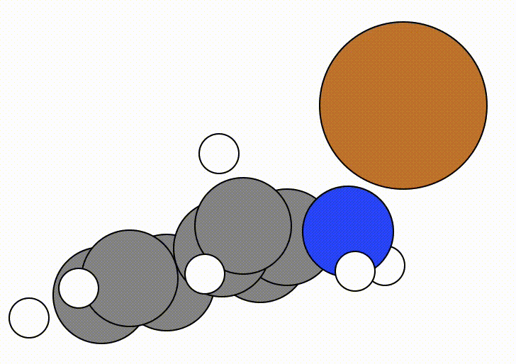
viewORCA append: Append Several Chemical Systems Together

This method is designed to allow the user to easily append multiple xyz files together into the same chemical system.

To use this module:

1. In the terminal, change directory into the directory containing the xyz files of the chemical systems you want to append together.

2. type viewORCA append filepath_for_system_1 filepath_for_system_2 filepath_for_system_3 ... into the terminal, where:

   • filepath_for_system_1, filepath_for_system_2, ... are the paths to all the xyz files you would like to append together.

The output file will be save into your current working directory as overall_chemical_system.xyz. CHange this filename to what you want it to be named.

Example

Lets consider an example where you want to append together a Cu(II)-benzylimine molecule (with centre of mass = (0.0,0.0,0.0)) with a benylamine molecule (with centre of mass = (10.0,0.0,0.0)) with a . We would run the code below to achieve this

# First, change directory into the folder containing your xyz files you want to append together. 
cd path_to_xyz_files

# Second, run "viewORCA move_com".
viewORCA append Benzylamine_com_10.0_0.0_0.0.xyz Cu_II-BnzImine_1+_com_0_0_0.xyz

You will see a new file has been made called overall_chemical_system.xyz that contains your overall chemical system. This example is given in Examples/viewORCA_append

Appending Benzylamine to the Cu(II)-benzylimine xyz file.